Using Stan Models: A Robust Linear Regression Example
We will approximate the posterior for the simple 2D robust linear regression model
and use Stan to compute (the gradient of) the model log density.
For more details and discussion of this example, see:
Practical posterior error bounds from variational objectives. Jonathan H. Huggins, Mikołaj Kasprzak, Trevor Campbell, Tamara Broderick. In Proc. of the 23rd International Conference on Artificial Intelligence and Statistics (AISTATS), Palermo, Italy. PMLR: Volume 108, 2020.
[1]:
import os
import pickle
import warnings
import matplotlib.pyplot as plt
import seaborn as sns
import autograd.numpy as np
import pystan

from viabel import bbvi, vi_diagnostics, MultivariateT
[2]:
# code for comparing to ground-truth posterior

sns.set_style('white')
sns.set_context('notebook', font_scale=1.5, rc={'lines.linewidth': 2})

def plot_approx_and_exact_contours(log_density, approx, var_param, cmap2='Reds'):
    xlim = [-4,-1]
    ylim = [-.5,3.5]
    xlist = np.linspace(*xlim, 100)
    ylist = np.linspace(*ylim, 100)
    X, Y = np.meshgrid(xlist, ylist)
    XY = np.concatenate([np.atleast_2d(X.ravel()), np.atleast_2d(Y.ravel())]).T
    zs = np.exp(log_density(XY))
    Z = zs.reshape(X.shape)
    zsapprox = np.exp(approx.log_density(var_param, XY))
    Zapprox = zsapprox.reshape(X.shape)
    cs_post = plt.contour(X, Y, Z, cmap='Greys', linestyles='solid')
    cs_post.collections[len(cs_post.collections)//2].set_label('Posterior')
    cs_approx = plt.contour(X, Y, Zapprox, cmap=cmap2, linestyles='solid')
    cs_approx.collections[len(cs_approx.collections)//2].set_label('Approximation')
    plt.xlim(xlim)
    plt.ylim(ylim)
    plt.legend()
    plt.show()

def check_accuracy(true_mean, true_cov, var_param, approx):
    approx_mean, approx_cov = approx.mean_and_cov(var_param)
    true_std = np.sqrt(np.diag(true_cov))
    approx_std = np.sqrt(np.diag(approx_cov))
    mean_error=np.linalg.norm(true_mean - approx_mean)
    cov_error_2=np.linalg.norm(true_cov - approx_cov, ord=2)
    cov_norm_2=np.linalg.norm(true_cov, ord=2)
    std_error=np.linalg.norm(true_std - approx_std)

    print('mean error             = {:.3g}'.format(mean_error))
    print('stdev error            = {:.3g}'.format(std_error))
    print('||cov error||_2^{{1/2}}  = {:.3g}'.format(np.sqrt(cov_error_2)))
    print('||true cov||_2^{{1/2}}   = {:.3g}'.format(np.sqrt(cov_norm_2)))
First, compile the robust regression Stan model:
[3]:
compiled_model_file = 'robust_reg_model.pkl'
try:
    with open(compiled_model_file, 'rb') as f:
        regression_model = pickle.load(f)
except:
    regression_model = pystan.StanModel(file='robust_regression.stan',
                                        model_name='robust_regression')
with open(compiled_model_file, 'wb') as f:
    pickle.dump(regression_model, f)
INFO:pystan:COMPILING THE C++ CODE FOR MODEL robust_regression_2f7d931ef1dc99d991576051801065c4 NOW.
Next, to as use a data, generate 25 observations from the model with \(\beta = (-2, 1)\):
[4]:
np.random.seed(5039)
beta_gen = np.array([-2, 1])
N = 25
x = np.random.randn(N, 2).dot(np.array([[1,.75],[.75, 1]]))
y_raw = x.dot(beta_gen) + np.random.standard_t(40, N)
y = y_raw - np.mean(y_raw)
For illustration purposes, generate ground-truth posterior samples using Stan’s dynamic HMC implementation:
[5]:
data = dict(N=N, x=x, y=y, df=40)
fit = regression_model.sampling(data=data, iter=50000, thin=50, chains=4)
true_mean = np.mean(fit['beta'], axis=0)
true_cov = np.cov(fit['beta'].T)
Standard mean-field variational inference
As a first example, we compute a mean field variational approximation using standard variational inference – that is, by maximimizing the evidence lower bound (ELBO):
[6]:
mf_results = bbvi(2, fit=fit, num_mc_samples=50)
average loss = 21.331 | R hat converged|: 17%|█▋ | 1737/10000 [00:09<00:45, 180.89it/s]
Convergence reached at iteration 1737
We can check approximation quality using vi_diagnostics, which determines the approximation is not good:
[7]:
mf_objective = mf_results['objective']
with warnings.catch_warnings():
    warnings.simplefilter('ignore')
    diagnostics = vi_diagnostics(mf_results['opt_param'], objective=mf_objective,
                                 n_samples=100000)
Pareto k is estimated to be khat = 0.91
WARNING: khat > 0.7 means importance sampling is not feasible.
WARNING: not running further diagnostics
Indeed, due to the strong posterior correlation, the variational approximation dramatically underestimates uncertainty:
[8]:
plot_approx_and_exact_contours(mf_objective.model, mf_objective.approx,
                               mf_results['opt_param'])
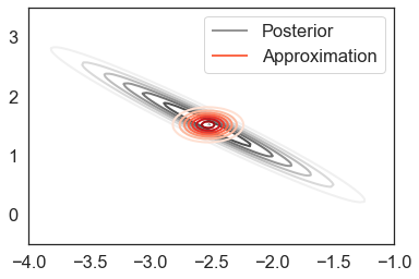
We can confirm the poor approximation quality numerically by examining the mean, standard deviation, and covariance errors as compared to the ground-truth estimates:
[9]:
check_accuracy(true_mean, true_cov, mf_results['opt_param'], mf_objective.approx)
mean error             = 0.00126
stdev error            = 0.73
||cov error||_2^{1/2}  = 0.919
||true cov||_2^{1/2}   = 0.93
An approximation with full covariance
To get a good approximation, we can instead use a Multivariate t variational family with a full-rank scaling matrix:
[10]:
t_results = bbvi(2, n_iters=2500, fit=fit, approx=MultivariateT(2, 100), num_mc_samples=100)
average loss = 23.096 | R hat converged|: 53%|█████▎ | 1316/2500 [00:18<00:16, 72.92it/s]
Convergence reached at iteration 1316
The diagnostics suggest the approximation is accurate:
[11]:
t_objective = t_results['objective']
with warnings.catch_warnings():
    warnings.simplefilter('ignore')
    diagnostics = vi_diagnostics(t_results['opt_param'], objective=t_objective,
                                 n_samples=100000)
Pareto k is estimated to be khat = -0.75

The 2-divergence is estimated to be d2 = 0.00069

All diagnostics pass.
Visual inspection and numerical checks confirm the diagnostics:
[12]:
plot_approx_and_exact_contours(t_objective.model, t_objective.approx, t_results['opt_param'])
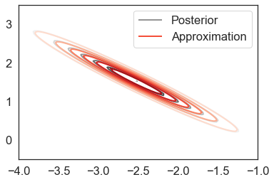
[13]:
check_accuracy(true_mean, true_cov, t_results['opt_param'], t_objective.approx)
mean error             = 0.00182
stdev error            = 0.00129
||cov error||_2^{1/2}  = 0.046
||true cov||_2^{1/2}   = 0.93